제어
제어 1 - 역기구학(IK)와 PID 이론
로봇 팔 제어의 핵심, 역기구학과 PID 이론을 파헤칩니다.
권민재
진행할 내용
매니퓰레이터에서의 엔드이펙터(EE) 제어방식을 예시로하여 역기구학(IK)과 PID 추총 알고리즘에 대해 학습하도록 하겠습니다.
이후 간단한 Matlab을 통한 실습을 통해 2자유도 2D제어 실습, 과제를 진행해보겠습니다.
역기구학(IK)이란?
매니퓰레이터를 보면 일반적으로 제어할때 (X, Y, Z) 3차원 좌표를 전달하여 EE가 이동하는것을 알 수 있습니다.
이러한 동작은 크게 두 단계로 나누어 볼 수 있습니다.
먼저 IK를 통해 목표 말단 좌표를 목표 관절각으로 변환하고,
이후 PID와 같은 하위 제어기를 통해 실제 모터가 목표 관절각을 추종하도록 만듭니다.
우선 이해를 쉽게하기 위해 2차원의 (X, Y) 매니퓰레이터가 있다고 가정하겠습니다.
원하는 좌표 (예시: 2, 2)로 가기 위한 과정을 살펴보면 2가지 문제가 보입니다.
1. (x, y) → (2, 2) 변환: 이 좌표에 도달하려면 각 관절은 몇 도여야 하나?
2. 현재 각도에서 목표 각도로 추종하기 위해 모터를 어떻게 움직여야되나?
1번이 IK, 2번이 PID에 해당하는 부분입니다.
먼저 역기구학(IK)에 대해 보도록하겠습니다.
역기구학이란 말 그대로 말단 좌표 값으로부터 관절각이 어떻게 구성되어야 하는지를 알아내는 방법이고,
정기구학은 각 관절의 각도와 길이를 알고 말단 좌표를 구하는 것입니다.
하지만 역기구학은 정기구학처럼 입력값만 받아서 쉽게 역산해낼 수 있는 구조가 아닙니다.
왜냐하면, 같은 말단좌표라고 하더라도 Case, 상황이 여러가지일 수 있고,
로봇의 복잡성이 증가하면서 답이 깔끔하게 떨어지는 Closed-form soulution이 나오지 않을 수 있습니다.
그래서 역기구학 또한 여러가지 하위 방법들로 나뉘어지고, 이를 조합하여 사용합니다.
그 중 대표적인 Closed-form (기하학적 풀이) 과, 일반화된 방법인 Jacobian Pseudoinverse (수치적 반복) 방식에 대해 알아보겠습니다.
A. Closed-form — 기하학적 풀이
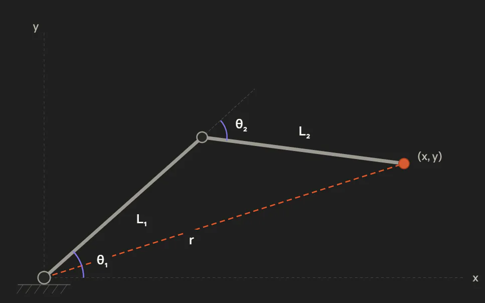
2-link arm처럼 단순한 구조에서는 삼각함수로 직접 풀 수 있습니다. 링크 길이를 L1, L2, 목표점을 (x, y)라 둘때
r² = x² + y²
cos(θ2) = (r² − L1² − L2²) / (2·L1·L2)
θ2 = ±acos(...)        # ± 두 해 = 팔꿈치 위/아래
θ1 = atan2(y, x) − atan2(L2·sin(θ2), L1 + L2·cos(θ2))
여기서 θ2의 ±가 앞서 말한 "같은 말단 좌표에 여러 해가 존재"하는 경우입니다. 팔꿈치를 위로 접든 아래로 접든 같은 점에 닿기 때문에,
두 개의 해가 동시에 존재합니다. 실제 구현에서는 상황에 맞게 하나를 골라 씁니다.
장점은 빠르고, 정확하고, 모든 해를 다 알 수 있습니다.
단점은 로봇 구조가 바뀌면 새로 유도해야 하며, 6자유도 산업용 로봇팔처럼 구조가 복잡해지면 closed-form이 항상 존재한다는 보장이 없습니다.
B. Jacobian Pseudoinverse — 수치적 반복해법
복잡한 로봇에서는 자코비안 행렬(Jacobian matrix) 을 씁니다. 자코비안 J는 관절 속도와 말단 속도의 관계를 나타내는 행렬입니다.
Closed-form 방식은 한번에 정답(각도)를 구해내는 방식이였습니다.
하지만 jacobian 방식은 한번에 정답을 구하는 방식이 아니라 각 관절을 조금씩 움직여보면서 말단목표로 가도록 계속 보정하는 방식입니다.
자코비안 행렬은 각 관절을 돌렸을때 말단의 좌표 값이 어떻게 움직이는가에 대한 데이터를 모아놓은 것으로 볼 수 있습니다.
[ x 변화 ]   [ θ1이 x에 주는 영향   θ2가 x에 주는 영향 ] [ θ1 변화 ]
[ y 변화 ] = [ θ1이 y에 주는 영향   θ2가 y에 주는 영향 ] [ θ2 변화 ]
수식으로는 다음과 같이 표현 할 수 있습니다.
Δx = J(q) · Δq Δx는 말단을 얼마나 움직이고 싶은지, Δq는 관절을 얼마나 움직일지를 나타냅니다.
그런데 이런 set이 현재 자세에서만 알맞는 근사치라는게 문제입니다.
로봇암은 여러관절로 이루어져있기 때문에 곡선으로 움직입니다, 하지만 여기서 곡선을 계속 확대해서 보면 직선처럼 보이게 할 수 있습니다.
바로 이러한 점에 착안하여 곡선으로 움직이는 것처럼 보이지만, 직선계산을 여러번 반복하면서 말단좌표를 따라가는 반복적 풀이인 것입니다.
자코비안도 역행렬을 구하지 못하는경우가 있습니다.
특이점이라고도 하는데, 어떤 경우일까요 (어느경우인지는 퀴즈🤔)
이럴때는 의사역행렬을 통해 해결합니다.
Δq = J⁺ · Δx말단에서 필요한 작은 이동량 Δx를 만들기 위해 각 관절을 얼마나 움직여야 하는지 Δq를 계산하는 식입니다.
정확한 역행렬을 만들 수 없을 때 가장 그럴듯한 관절 변화량을 계산해주는 일반화된 역행렬입니다.
정방행렬이면서 정칙일 때는 일반 역행렬과 같은 값이 나오고, 그렇지 않을 때 다음 3가지로 동작합니다.
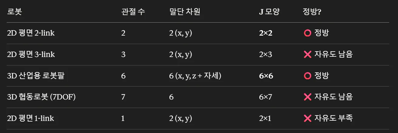
자유도가 부족할 때 → 목표에 정확히 도달할 수 없으니, 가장 가까이 갈 수 있는 해를 찾아줍니다. (작업공간 밖으로 나간경우)
자유도가 남을 때 → 같은 목표에 도달하는 관절 조합이 여러 개 존재하므로, 그중 움직임이 가장 작은 해를 골라줍니다. (같은 점에 닿는 자세가 무수히 많은경우)
특이점일 때 → J⁺도 발산. DLS 같은 보완이 필요. (팔이 완전히 펴진 자세)
J⁺  :  Δq = (J·Jᵀ)⁻¹ 같은 걸 푸는 과정
DLS :  Δq = Jᵀ(J·Jᵀ + λ²I)⁻¹ · Δx
                      ↑
                  여기 λ²I 더해줌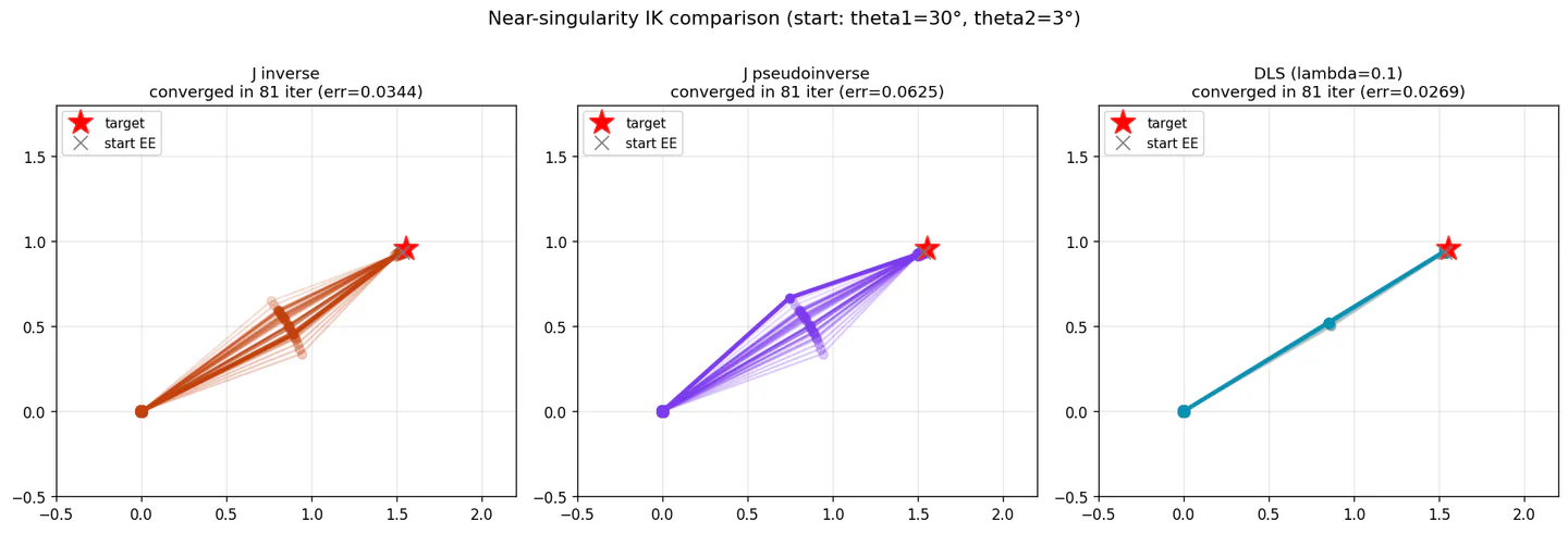
따라서 자코비안 기반 IK는 자유도 불일치 상황에서도 해를 계산할 수 있고 불안정성을 완화할 수 있어, 매니퓰레이터 제어에서 표준적으로 사용됩니다.
과제⭐⭐⭐⭐⭐
2-link 로봇팔 자코비안 IK 구현하기
목표: 자코비안J⁻¹ 행렬방식을 이용해 2-link 평면 로봇팔이 목표 좌표에 도달하도록 만들고,
특이점 근처에서 두 방식의 차이를 알아보기

환경
Python (numpy, matplotlib) 또는 MATLAB 중 선택
스켈레톤 코드 제공 (Slack)에 별도로 공유드리겠습니다!
제출물
완성된 코드 파일
보고서 (노션페이지에 실행 결과 영상 추가하여 1-2페이지 정리한 뒤 Slack에 공유해주세요 )
- 왜 이 자세가 특이점인지 작성하기
- 의사역행렬, DLS를 적용했을때 특이점에서 해결되는지 확인해보기
Control 1 - Inverse Kinematics (IK) and PID Theory
We delve into the core principles of robotic arm control: inverse kinematics and PID theory.
Agenda
Using the control method for an end-effector (EE) on a manipulator as an example, we will learn about inverse kinematics (IK) and PID tracking algorithms.
Following this, we will conduct a 2-DOF 2D control lab and complete an assignment through a simple hands-on exercise using MATLAB.
What is Inverse Kinematics (IK)?
When controlling a manipulator, we typically provide 3D coordinates (X, Y, Z) to move the end-effector (EE).
This process can be broadly divided into two stages.
First, inverse kinematics (IK) is used to convert the target end-effector coordinates into target joint angles.
Then, a sub-controller such as a PID controller is used to make the actual motor track the target joint angles.
To make it easier to understand, let’s assume we have a 2D (X, Y) manipulator.
When examining the process of reaching a desired coordinate (e.g., 2, 2), two problems become apparent.
1. (x, y) → (2, 2) transformation: What angles must each joint be at to reach this coordinate?
2. How should the motor be driven to track from the current angle to the target angle?
The first corresponds to IK, and the second corresponds to PID.
First, let’s look at inverse kinematics (IK).
Inverse kinematics is, quite literally, a method for determining how joint angles should be configured based on the end-effector coordinates, whereas
forward kinematics involves calculating the end-effector coordinates given the angles and lengths of each joint.
However, inverse kinematics is not structured like forward kinematics, where it can easily compute the solution based solely on input values.
This is because even for the same end-effector coordinates, there can be various cases and situations, and as the robot’s complexity increases, a clean closed-form solution may not be available.
Therefore, inverse kinematics is also divided into various sub-methods, which are combined and used.
Among these, we will explore the representative closed-form (geometric solution) method and the generalized Jacobian pseudoinverse (numerical iterative) method.
A. Closed-form — Geometric Solution
For simple structures like a 2-link arm, the problem can be solved directly using trigonometric functions. Given the link lengths L1, L2and the target point (x, y),
r² = x² + y²
cos(θ2) = (r² − L1² − L2²) / (2·L1·L2)
θ2 = ±acos(...)        # ± 두 해 = 팔꿈치 위/아래
θ1 = atan2(y, x) − atan2(L2·sin(θ2), L1 + L2·cos(θ2))
Here, θ2is ±is an example of the previously mentioned case where "multiple solutions exist for the same end-point coordinates." Since the arm touches the same point whether the elbow is bent upward or downward, two solutions exist simultaneously. In actual implementation, one is selected and used depending on the situation.
The advantages are that it is fast, accurate, and provides all possible solutions.
The disadvantages are that it must be derived anew if the robot structure changes, and there is no guarantee that a closed-form solution will always exist as the structure becomes more complex, such as in a 6-DOF industrial robot arm.
B. Jacobian Pseudoinverse — Numerical Iterative Method
For complex robots, the Jacobian matrix is used. The Jacobian Jis a matrix that represents the relationship between joint velocities and end-effector velocity.
The closed-form method directly calculates the exact solution (angles) in a single step.
However, the Jacobian method does not calculate the exact solution immediately; instead, it continuously adjusts the path by moving each joint slightly to reach the end-effector target.
The Jacobian matrix can be viewed as a collection of data describing how the end-effector’s coordinates change when each joint is rotated.
[ x 변화 ]   [ θ1이 x에 주는 영향   θ2가 x에 주는 영향 ] [ θ1 변화 ]
[ y 변화 ] = [ θ1이 y에 주는 영향   θ2가 y에 주는 영향 ] [ θ2 변화 ]
Mathematically, this can be expressed as follows.
Δx = J(q) · Δq Δx represents how much we want to move the end effector, and Δq represents how much to move the joints.
However, the problem is that this set is only an approximation valid for the current pose.
Since a robotic arm consists of multiple joints, it moves in a curved path; however, if we continuously zoom in on this curve, we can make it appear as a straight line.
Drawing on this insight, the solution is an iterative process that, while appearing to move in a curved path, actually follows the end-effector coordinates by repeatedly performing linear calculations.
There are also cases where the Jacobian cannot be inverted.
These are called singularities—but in what situations do they occur? (That’s a quiz for you 🤔)
In such cases, we solve the problem using the pseudo-inverse matrix.
Δq = J⁺ · ΔxThis is a formula for calculating Δq—the amount each joint must move—to achieve the small displacement Δx required at the end point.
It is a generalized inverse matrix that calculates the most plausible joint displacements when an exact inverse matrix cannot be constructed. When the matrix is square and regular, it yields the same values as the standard inverse matrix; otherwise, it operates in the following three ways.
When there are insufficient degrees of freedom → Since the target cannot be reached exactly, it finds the solution that gets closest to it. (When the joint moves outside the workspace)
When there are extra degrees of freedom → Since there are multiple joint combinations that reach the same goal, it selects the solution with the smallest movement. (When there are countless poses that reach the same point)
When a singularity occurs → J⁺ also diverges. A supplement like DLS is required. (When the arm is fully extended)
J⁺  :  Δq = (J·Jᵀ)⁻¹ 같은 걸 푸는 과정
DLS :  Δq = Jᵀ(J·Jᵀ + λ²I)⁻¹ · Δx
                      ↑
여기 λ²I 더해줌Therefore, Jacobian-based IK can compute solutions even in situations of degree-of-freedom mismatch and mitigate instability, making it the standard method used in manipulator control.
Assignment⭐⭐⭐⭐⭐
Implementing Jacobian IK for a 2-link robotic arm
Objective: Use the Jacobian J⁻¹ matrix method to make a 2-link planar robotic arm reach the target coordinates, and examine the differences between the two methods near singularities
Environment
Choose between Python (numpy, matplotlib) or MATLAB
I will share the skeleton code separately on Slack!
Submission
Completed code file
Report (Please summarize your findings in 1–2 pages on a Notion page, including a video of the execution results, and share it on Slack.
) - Explain why this pose is
a singularity. - Check whether applying the inverse matrix and DLS resolves the singularity.