제어
제어 3 - 역기구학 수식 직접 풀기 + PID
2링크 로봇팔을 예로 들어, 목표 좌표를 관절각으로 바꾸는 방법과 실제 모터가 그 각을 따라가는 과정을 차근차근 살펴봅니다.
권민재
들어가며
이번 글의 목표는 로봇팔의 손을 원하는 좌표로 보내는 계산을, 식이 왜 필요한지부터 차근차근 확인해봅니다.
FK — 관절각을 알 때 손의 위치를 구합니다.
Closed-form — 목표 손 위치에서 관절각을 한 번에 구합니다.
Jacobian — 목표를 향해 조금씩 움직일 관절 변화량을 구합니다.
의사역행렬과 DLS — 팔이 너무 펴진 자세에서도 변화량이 과해지지 않게 합니다.
PID — 계산된 목표 관절각까지 실제 모터를 움직입니다.
전제는 2링크 평면 로봇팔입니다. 링크 길이는
어깨(θ₁) ── L₁ ── 팔꿈치(θ₂) ── L₂ ── 손(x, y)0. 출발점 — 정기구학(FK) 세우기
먼저 답할 질문은 이것입니다.
“어깨와 팔꿈치를 이 각도로 놓으면, 손, EE은 어디에 있는가?”
이 질문에 답하는 식이 정기구학, 즉 FK입니다. 링크 1이 만드는 팔꿈치 위치에 링크 2가 더하는 위치를 합치면 손의 최종 위치가 됩니다.
예를 들어
1. Closed-form — 코사인 법칙으로 직접 풀기
이번에는 질문을 반대로 생각해봅니다.
“손을
에 두려면 관절은 몇 도여야 하는가?”
2링크 평면 팔은 코사인 법칙을 이용해 이 답을 한 번에 구할 수 있습니다. 먼저 어깨에서 목표점까지의 거리 제곱을 둡니다.
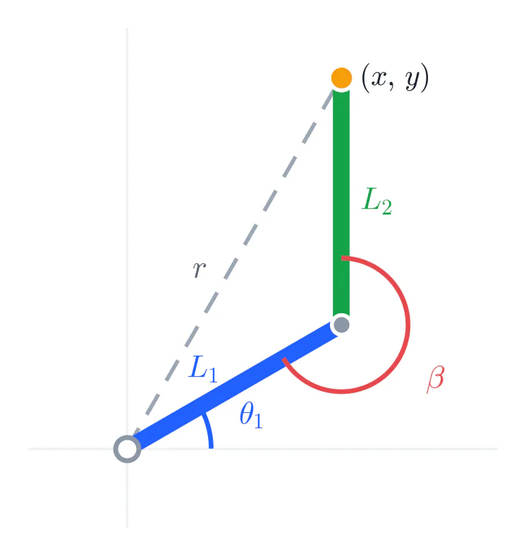
코사인 법칙으로 팔꿈치 각도의 코사인값을 구합니다.
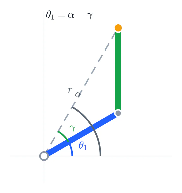
팔꿈치 각도를 얻으면, 목표점을 향한 방향에서 링크 2가 차지하는 각을 빼 어깨 각도를 구합니다.
1-3. 숫자로 확인 — 깔끔한 예시
따라서 한 해에서는
가 됩니다. 즉 어깨는
Closed-form은 빠르고 정확합니다. 다만 링크 수가 많아지거나 관절 제한, 장애물 회피 같은 조건이 늘어나면 식을 직접 만들기 어려워집니다.
2. Jacobian — 미분으로 만드는 일반 해법
이번에는 정답을 한 번에 구하지 않고 목표를 향해 조금씩 다가가 보겠습니다.
“손을 아주 조금 오른쪽이나 위쪽으로 옮기려면, 어느 관절을 얼마나 돌려야 하는가?”
Jacobian
: 손이 움직여야 할 작은 거리 : 관절이 움직여야 할 작은 각도 : 현재 자세에서 관절 움직임을 손 움직임으로 바꾸는 표
FK 식을
2-2. 거꾸로 풀기 — 역행렬과 행렬식
손의 목표 방향
단, 역행렬은 존재할 때만 쓸 수 있습니다. 2링크 팔에서는 행렬식이
입니다. 이 값이 0에 가까우면 팔이 펴지거나 접힌 특이점에 가까워졌다는 신호입니다.
2-3. 정사각이 아니거나 특이점일 때 — 의사역행렬과 DLS
역행렬을 쓸 수 없거나 불안정할 때는 의사역행렬을 사용합니다.
의사역행렬은 가능한 한 목표에 가깝게 가면서 관절 움직임도 작은 답을 고릅니다. 하지만 특이점에 아주 가까우면 이 방법도 큰 관절 변화량을 만들 수 있습니다. 이때는 DLS로 계산식을 완화합니다.
3. 행렬이 한 스텝마다 어떻게 굴러가나 — 숫자로
이제 실제 숫자를 넣어 보겠습니다.
FK로 구한 현재 손 위치는
즉 손은 조금 오른쪽, 조금 아래로 가야 합니다. 이 자세의 Jacobian은
이고, 이를 거꾸로 풀면
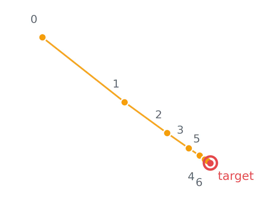
현재 손 위치 계산
→ 목표와의 오차 계산
→ 현재 자세의 J 계산
→ Δq 계산
→ 관절각 갱신
→ 반복
이 과정을 반복하면 오차는 약
4. 특이점에서 무슨 일이 — 숫자로 본 pinv vs DLS
팔이 완전히 펴지거나 접히면
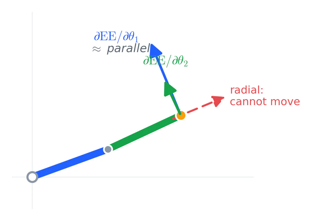
예를 들어 거의 펴진 자세에서는 의사역행렬이 작은 손 이동에
즉 DLS는 특이점 근처에서 “목표를 향해 가되, 너무 큰 걸음은 걷지 말자”라고 계산하는 댐핑 방법입니다.
5. PID — 목표 관절각을 실제로 추종하기
Closed-form은 목표 관절각을 한 번에 구하고, Jacobian IK는 관절 변화량을 반복해 목표 자세에 가까워집니다. 그러나 실제 로봇에서는 모터가 그 목표 각도까지 움직여야 합니다. 그 일을 PID가 담당합니다.
P: 아직 얼마나 모자라는지 보고 밀어 줍니다.
I: 오래 남아 있던 작은 오차까지 모아 없앱니다.
D: 목표를 지나치지 않도록 브레이크를 겁니다.
error = target_angle - current_angle
integral += error * dt
derivative = (error - previous_error) / dt

motor_command = Kp * error + Ki * integral + Kd * derivative
전체 흐름은 목표 손 위치 → Closed-form 또는 반복형 Jacobian IK → 목표 관절각 → PID → 실제 모터입니다. Jacobian IK에서는 매 반복의
마무리
FK는 관절각에서 손 위치를 구합니다.
Closed-form은 목표 위치에서 관절각을 한 번에 구합니다.
Jacobian은 손의 작은 오차를 관절의 작은 변화량으로 바꿉니다.
DLS는 특이점 근처에서 관절 변화량을 완화합니다.
PID는 목표 관절각을 실제 모터가 따라가게 합니다.
Closed-form은 빠르게 정답을 구하는 공식이고, Jacobian은 목표로 조금씩 다가가는 지도이며, DLS는 특이점 근처의 댐핑 장치이고, PID는 실제 모터를 움직이는 운전 방법이다.
실습 과제 — 브라우저 시뮬레이터
위에서 유도한 식을 그대로 코드로 옮겨, 2링크 로봇팔이 목표를 따라가게 만들어 봅니다. 설치 없이 브라우저에서 바로 실행됩니다. 학생이 채우는 ik_step(q, target) 함수 한 번의 호출이 3장의 한 스텝입니다.
목표 — 스켈레톤의
ik_step(q, target)를 채워 자코비안 IK를 구현하고, 팔이 목표 좌표에 수렴하게 만들기비교 — 특이점 근처에서 pseudoinverse와 DLS의 차이를 “특이점 예제”로 확인하기
응용 — Pick & Place 모드에서 집기 → 옮기기 → 놓기를 수행하기
제출물 — 완성 코드, 실행 결과(영상 또는 스크린샷), 특이점에서 pinv와 DLS를 비교한 1–2쪽 보고서
▶ 시뮬레이터 열기 — 첫 로딩만 인터넷이 필요하며 몇 초 걸릴 수 있습니다.
Control 3 - Working Through the IK Math + PID
Deriving the inverse-kinematics formulas by hand — from the law of cosines to the Jacobian — and tracing Jacobian IK one numeric step at a time, ending with PID tracking.
Introduction
Part 1 covered what inverse kinematics (IK) is and why it is hard, and introduced the two branches — closed-form and Jacobian — at a conceptual level.
This post follows, by hand, where those result formulas actually come from. Starting from a single line of the law of cosines, we trace every step: how the Jacobian matrix is re-filled with concrete numbers at each iteration and how the error shrinks. At the end we also derive the PID controller that was only in Part 1's title but missing from its body.
Setup: a 2-link planar manipulator (two links, 2 planar DOF). Link lengths
, joint angles . All angles are in radians.
0. Starting point — Forward Kinematics (FK)
To solve inverse kinematics we first need forward kinematics. Once we write down "where the end-effector goes given the angles," both the closed-form and the Jacobian solutions follow by manipulating or differentiating this one expression.
Joint 1 is at the origin;
To shorten notation, write
Now we invert this expression two ways in turn: first the closed form that gives the answer in one shot, then the iterative Jacobian method that approaches it gradually.
1. Closed-form — solving directly with the law of cosines
The goal is reversed: given a target EE position
1-1.
Consider the triangle with vertices at the origin, the elbow, and the EE. Its three sides have lengths
Let
But the joint angle
Substituting flips the sign and tidies up:
This is exactly the formula Part 1 stated without derivation. The angle is
The
1-2.
Grouping the FK expression by
Substitute into
Letting
A rotation adds angles, so the direction angle of the target vector equals "
Therefore
Once you pick the sign of
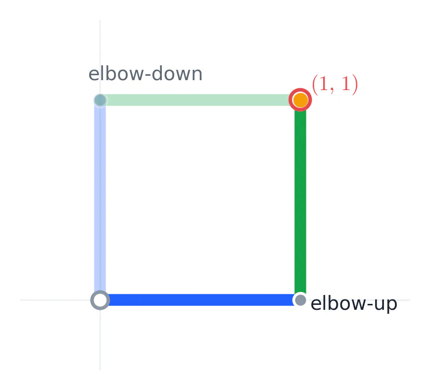
1-3. Checking with numbers — a clean example
Let
r²      = 1² + 1² = 2
cosθ2   = (2 − 1 − 1) / (2·1·1) = 0
θ2      = ±90°        (up / down, two solutions)

[elbow-up]  θ2 = +90°
θ1 = atan2(1,1) − atan2(1·sin90°, 1 + 1·cos90°)
   = 45° − atan2(1, 1) = 45° − 45° = 0°
check (FK):  x = cos0° + cos(0°+90°) = 1 + 0 = 1  ✓
            y = sin0° + sin(0°+90°) = 0 + 1 = 1  ✓

[elbow-down]  θ2 = −90°
θ1 = 45° − atan2(−1, 1) = 45° − (−45°) = 90°
check (FK):  x = cos90° + cos(90°−90°) = 0 + 1 = 1  ✓
            y = sin90° + sin(0°)       = 1 + 0 = 1  ✓
Both solutions land exactly on
Pros: one exact answer in one shot, and it gives all solutions. Cons: change the structure and you must re-derive from scratch, and for complex arms (e.g. 6-DOF) such a clean formula is not guaranteed to exist. Hence we need a general method.
2. Jacobian — a general method via differentiation
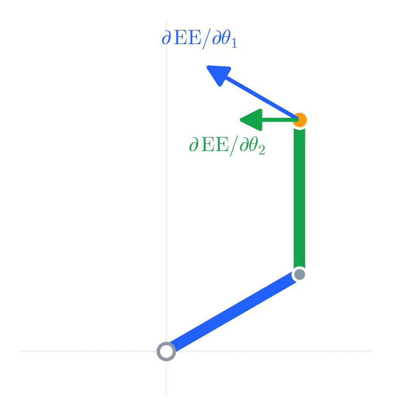
If closed-form "solves for the angles directly," the Jacobian method "nudges toward the target a little at a time." The key is to differentiate FK with respect to the angles to build a matrix describing "how the EE moves when each joint turns a bit."
2-1. Filling in
The Jacobian is the
Differentiate
∂x/∂θ1 = −L1 s1 − L2 s12      (d/dθ1 of c12 → −s12)
∂x/∂θ2 =        − L2 s12      (d/dθ2 of c12 → −s12; L1 term has no θ2)
∂y/∂θ1 =  L1 c1 + L2 c12
∂y/∂θ2 =          L2 c12
Collecting:
This matrix links joint velocity to EE velocity. In differential form it is Part 1's relation:
2-2. Inverting — the inverse matrix and the determinant
We want the reverse: "to move the EE by
Let us expand the determinant fully (this result is exactly what flags singularities):
The
This one line answers Part 1's quiz ("when can the Jacobian not be inverted?").
2-3. When non-square or singular — pseudoinverse and DLS
At a singularity, or when the matrix is non-square (mismatched DOF), an ordinary inverse does not exist. Then we use the pseudoinverse
For a square, nonsingular matrix the pseudoinverse gives exactly the same value as the ordinary inverse. To make that concrete: for the first pose used in Section 3,
They differ when not full rank. There
Adding
3. How the matrix rolls each step — with numbers
Now the part we most wanted to see. As Jacobian IK iterates step by step, we trace exactly what numbers fill the matrix and how the error shrinks.
Setup:
Step 0 — fill
q0 = (30°, 60°)
current EE = (cos30°+cos90°, sin30°+sin90°) = (0.866, 1.500)
error Δx = target − EE = (1.0−0.866, 1.4−1.500) = (0.1340, −0.1000)
|Δx| = √(0.1340² + 0.1000²) = 0.1672

fill the Jacobian "at this pose":
s1=sin30°=0.5,  c1=cos30°=0.866,  s12=sin90°=1,  c12=cos90°=0
J = [ −0.5−1   −1 ] = [ −1.5   −1 ]
    [  0.866   0 ]     [ 0.866   0 ]
det J = L1·L2·sin60° = 0.866      (≠0 → inverse exists)

J⁻¹ = (1/0.866)·[ 0      1   ] = [  0      1.155 ]
                [ −0.866 −1.5 ]   [ −1.0   −1.732 ]

full correction  J⁻¹·Δx = (−0.1155, +0.0392) rad
apply step       α·J⁻¹·Δx = 0.5·(−0.1155, 0.0392) = (−0.0578, +0.0196) rad
                                                  = (−3.31°, +1.12°)     ← rad × 180/π
q1 = q0 + α·Δq = (30−3.31, 60+1.12) = (26.69°, 61.12°)
Step 1 — re-fill the same matrix (the numbers change)
q1 = (26.69°, 61.12°)
EE = (0.9315, 1.4485),   error |Δx| = 0.0839   (about half of step 0's 0.1672)

recompute J at the new pose → every entry changes:
J = [ −1.4485  −0.9993 ]    det J = L1·L2·sin(61.12°) = 0.8757
    [  0.9315   0.0381 ]
Δx = (0.0685, −0.0485)
α·J⁻¹·Δx = (−1.50°, +0.21°)
q2 = (25.19°, 61.33°)
The key point:
Steps 0–6 — watching the error shrink
step |  θ1(°)    θ2(°)  |   EE (x, y)        |   error
  0  |  30.000  60.000  |  (0.8660, 1.5000)  |  0.16718
  1  |  26.692  61.124  |  (0.9315, 1.4485)  |  0.08388
  2  |  25.193  61.334  |  (0.9655, 1.4238)  |  0.04197
  3  |  24.485  61.353  |  (0.9827, 1.4118)  |  0.02099
  4  |  24.141  61.341  |  (0.9913, 1.4059)  |  0.01049
  5  |  23.972  61.330  |  (0.9956, 1.4029)  |  0.00525
  6  |  23.888  61.323  |  (0.9978, 1.4015)  |  0.00262
With
As an algorithm:
repeat:
    Δx = x_target − FK(q)          # remaining error
    if |Δx| < tolerance: break
    J  = jacobian(q)               # re-filled at the current pose
    Δq = pinv(J) · Δx              # (use DLS near a singularity)
    q  = q + α · Δq                # α: step size (0<α≤1)
The simulator assignment opens in exactly this state — start
, target , — so the table above plays out on screen. One call of the ik_step(q, target)function you implement is one step above, and the on-screendet(J)=L1·L2·sinθ2readout is the very value derived in Section 2-2.
4. What happens at a singularity — pinv vs DLS in numbers
Now the DLS we deferred in Section 2-3, in numbers. Push
q = (20°, 5°)   →   EE = (1.846, 0.765)
J = [ −0.765  −0.423 ]    det J = sin5° = 0.0872   →   1/detJ = 11.47 (amplified!)
    [  1.846   0.906 ]

want to push the EE outward (radially) by just 0.05 (5% of a link length):
Δx = (0.046, 0.019),  |Δx| = 0.05

[pseudoinverse]  Δq = pinv(J)·Δx = (32.8°, −65.7°)   |Δq| = 1.28 rad
                 → tens of degrees of joint motion for a tiny 0.05 move (blow-up)

[DLS, λ=0.1]     Δq = J ᵀ(J J ᵀ + λ²I)⁻¹·Δx = (4.3°, −8.7°)   |Δq| = 0.17 rad
                 → same target, ~7× smaller joint change, stable
For the same
5. PID — actually tracking the target joint angle
Once IK has given a "target joint angle
P (proportional) — pushes in proportion to the error. Larger is faster but too large oscillates. P alone usually leaves a small steady-state error.
I (integral) — integrates accumulated error to remove that steady-state error. Too much causes overshoot or integral windup.
D (derivative) — reacts to the rate of change of error, acting as a brake. It reduces overshoot and oscillation but is sensitive to measurement noise.
To run it in code we need the discrete form. At each time step
e_k        = θ_target − θ_k
integral  += e_k · Δt                      # accumulate integral
derivative = (e_k − e_{k−1}) / Δt          # finite-difference derivative
u_k        = Kp·e_k + Ki·integral + Kd·derivative
# apply u_k to the motor → θ updates → repeat next step
Tuning intuition: raise
Big picture: IK converts target coordinates → target joint angles, and PID makes the motor actually track those angles. Part 1's two problems (coordinates→angles / tracking the angle) map respectively here.
Wrap-up
In summary — closed-form gives
Now it is your turn to run it. The accompanying assignment ports the formulas above into code and watches a 3D robot arm follow the target in a browser simulator. Implement one ik_step of Section 3 yourself, and see the difference between the pseudoinverse and DLS at a singularity with your own eyes. (The simulator and assignment details are attached at the end of this post or provided separately.)
Assignment — Browser Simulator
Port the formulas derived above into code and make the 2-link arm follow a target — no install, it runs right in the browser (Python + numpy execute in-browser).
Goal — fill in the skeleton’s
ik_step(q, target)to implement Jacobian IK so the arm converges to the target (one step of Section 3 = one call of this function).Compare — see the difference between the pseudoinverse and DLS near a singularity (Section 4); the “singularity example” button reproduces it in one click.
Apply — switch to Pick & Place mode and check that the same
ik_stepperforms pick → carry → place.Submit — your finished code + a run recording/screenshots + a 1–2 page report (pinv vs DLS at a singularity).
▶ Open the simulator — only the first load needs internet and takes a few seconds.